library(tidyverse)Transcriptomics profiling of Ovarian Cancer cells
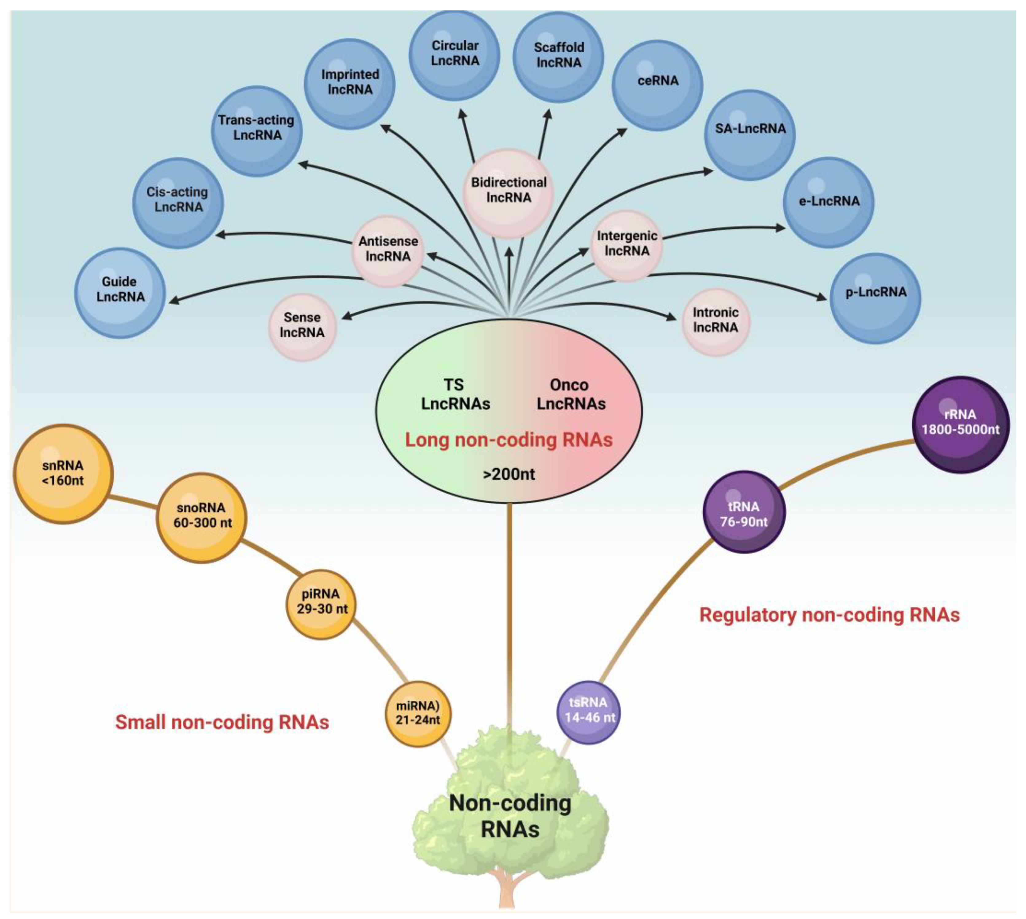
Introduction to long non-coding RNA
Long non-coding RNAs (lncRNAs) are RNA molecules that are longer than 200 nucleotides and do not code for proteins. Once considered “junk” in the genome, lncRNAs are now recognized as crucial regulators of gene expression. They can influence cellular processes such as chromatin remodeling, transcription, splicing, and translation by interacting with DNA, RNA, or proteins.
The goal of this study is to explore the transcriptomic changes in ovarian cancer cells by analyzing mRNA and lncRNA expression. We aim to identify significantly dysregulated genes and understand their roles in cancer progression using various computational techniques such as volcano plots, bar graphs, and PCA analysis.
What are the differentially expressed genes in Ovarian Cancer?
Preparing the data for volcano plot (mRNA Data)
mRNA_data <- read_csv("CNC_mRNA.csv")
mRNA_data <- mRNA_data |>
  mutate(
    log2FC = ifelse(Regulation == "down", -log2(FoldChange), log2(FoldChange)),
    negLog10P = -log10(p_value),
    status = case_when(
      log2FC >= 2 & p_value < 0.05 ~ "Upregulated",
      log2FC <= -2 & p_value < 0.05 ~ "Downregulated",
TRUE ~ "Not Significant"))table(mRNA_data$status)
  Downregulated Not Significant     Upregulated
            304            1290             380
Plotting the Volcano plot for mRNA data
ggplot(mRNA_data, aes(x = log2FC, y = negLog10P, color = status)) +
  geom_point(alpha = 0.8, size = 1.5) +
  scale_color_manual(values = c(
    "Upregulated" = "red",
    "Downregulated" = "green",
    "Not Significant" = "grey"
  )) +
  geom_vline(xintercept = c(-2, 2), linetype = "dotted", color = "black") +
  geom_hline(yintercept = -log10(0.05), linetype = "dotted", color = "black") +
  theme_minimal() +
  labs(
    title = "Differential mRNA Expression",
    x = "log2(Fold Change)",
    y = "-log10(p-value)"
  )
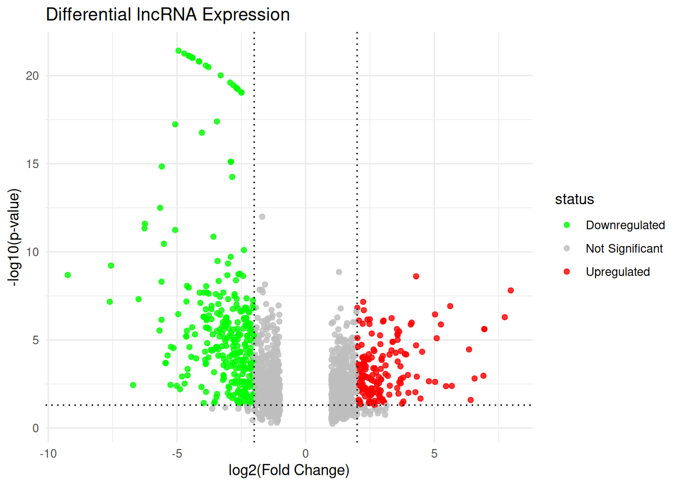
Preparing the data for volcano plot (lncRNA Data)
lncRNA_data <- read_csv("CNC_lncRNA.csv")
lncRNA_data <- lncRNA_data |>
  mutate(
    log2FC = ifelse(Regulation == "down", -log2(`FoldChange`), log2(`FoldChange`)),
    negLog10P = -log10(p_value),
    status = case_when(
      log2FC >= 2 & p_value < 0.05 ~ "Upregulated",
      log2FC <= -2 & p_value < 0.05 ~ "Downregulated",
      TRUE ~ "Not Significant"))
Preparing the data for volcano plot (lncRNA)
table(lncRNA_data$status)
  Downregulated Not Significant     Upregulated
            320            1440             172
Plotting the Volcano plot for lncRNA data
ggplot(lncRNA_data, aes(x = log2FC, y = negLog10P, color = status)) +
  geom_point(alpha = 0.8, size = 1.5) +
  scale_color_manual(values = c(
    "Upregulated" = "red",
    "Downregulated" = "green",
    "Not Significant" = "grey"
  )) +
  geom_vline(xintercept = c(-2, 2), linetype = "dotted", color = "black") +
  geom_hline(yintercept = -log10(0.05), linetype = "dotted", color = "black") +
  theme_minimal() +
  labs(
    title = "Differential lncRNA Expression",
    x = "log2(Fold Change)",
    y = "-log10(p-value)"
  )
What are the top twenty most upregulated and downregulated genes?
Top 20 upregulated mRNA
top_up_mRNA <- mRNA_data |> arrange(desc(log2FC)) |> slice_head(n = 20)Plot upregulated mRNA
ggplot(top_up_mRNA, aes(x = reorder(GeneSymbol, log2FC), y = log2FC, fill = negLog10P)) + geom_col() + scale_fill_gradient(low = "pink", high = "darkred", name = "-log10(p-value)") + coord_flip() + labs( title = "Top 20 Upregulated mRNA", x = "Gene Symbol", y = "log2(Fold Change)")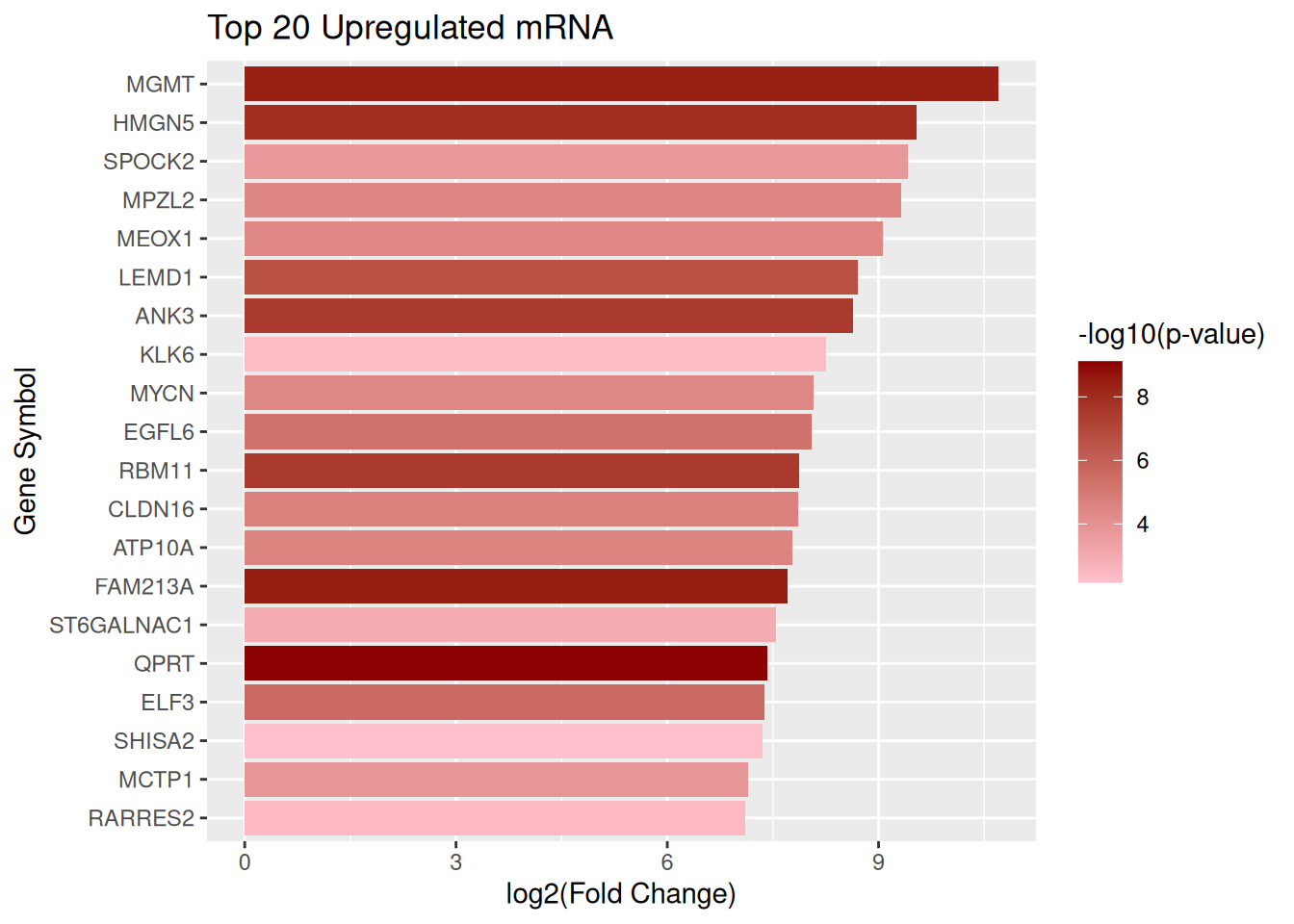
Top 20 downregulated mRNA
top_down_mRNA <- mRNA_data |> arrange(log2FC) |> slice_head(n = 20)Plot downregulated mRNA
ggplot(top_down_mRNA, aes(x = reorder(GeneSymbol, log2FC), y = log2FC, fill = negLog10P)) + geom_col() + scale_fill_gradient(low = "lightgreen", high = "darkgreen", name = "-log10(p-value)") + coord_flip() + labs(title = "Top 20 Downregulated mRNA", x = "Gene Symbol", y = "log2(Fold Change)")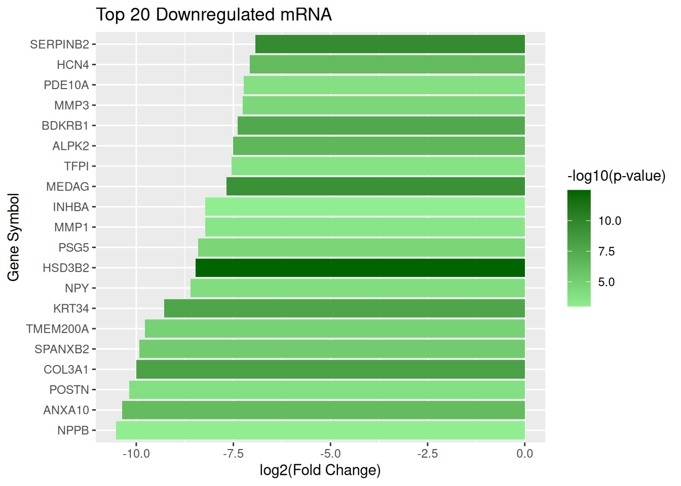
Top 20 upregulated lncRNA
top_up_lncRNA <- lncRNA_data |> arrange(desc(log2FC)) |> slice_head(n = 20)
ggplot(top_up_lncRNA, aes(x = reorder(GeneSymbol, log2FC), y = log2FC, fill = negLog10P)) + geom_col() + scale_fill_gradient(low = "pink", high = "darkred", name = "-log10(p-value)") + coord_flip() + labs( title = "Top 20 Upregulated lncRNA", x = "Gene Symbol", y = "log2(Fold Change)")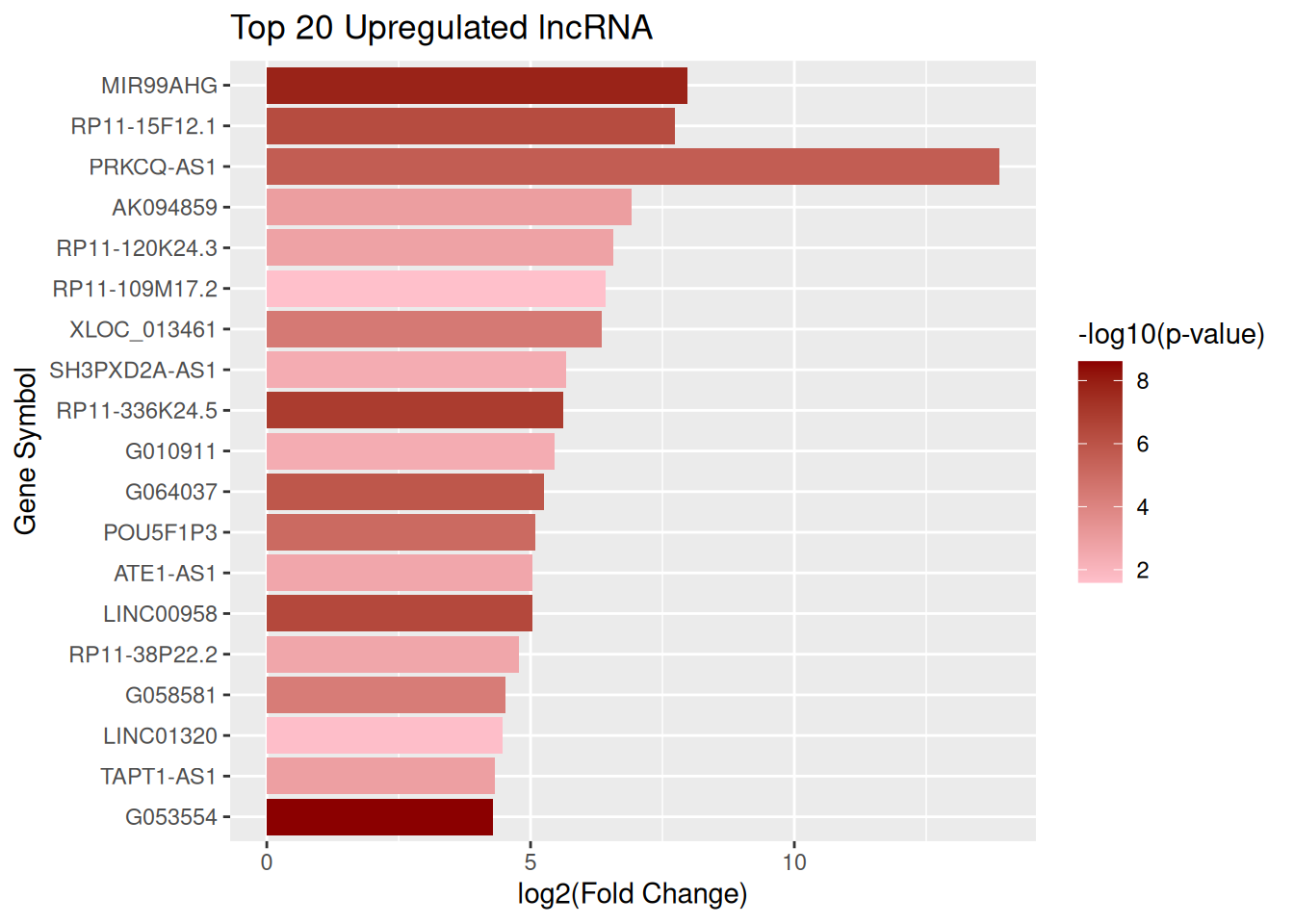
Top 20 downregulated lncRNA
top_down_lncRNA <- lncRNA_data |> arrange(log2FC) |> slice_head(n = 20)
ggplot(top_down_lncRNA, aes(x = reorder(GeneSymbol, log2FC), y = log2FC, fill = negLog10P)) + geom_col() + scale_fill_gradient(low = "lightgreen", high = "darkgreen", name = "-log10(p-value)") + coord_flip()  + labs(title = "Top 20 Downregulated lncRNA", x = "Gene Symbol", y = "log2(Fold Change)")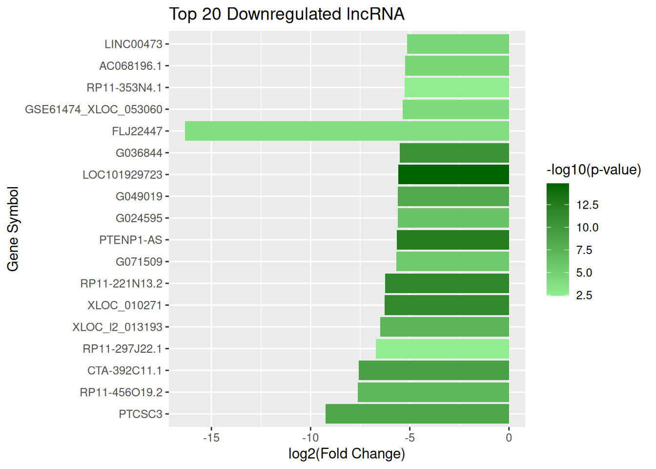
Is there any transcriptomic variation among the ovarian cancer samples and control sample?
lncRNA_data <- read_csv("CNC_lncRNA.csv")
mRNA_data <- read_csv("CNC_mRNA.csv")


expr_cols <- c("2,treatednormalized", "3,treatednormalized", "4,treatednormalized",
               "5,treatednormalized", "6,treatednormalized", "1,controlnormalized")

lncRNA_expr <- lncRNA_data[, expr_cols]
mRNA_expr <- mRNA_data[, expr_cols]
rownames(lncRNA_expr) <- make.unique(lncRNA_data$GeneSymbol)
rownames(mRNA_expr) <- make.unique(mRNA_data$GeneSymbol)
combined_expr <- rbind(mRNA_expr, lncRNA_expr)
combined_expr_t <- t(combined_expr)


rownames(combined_expr_t) <- c("Kuramochi", "SNU-119", "OVCAR3", "SKOV3", "OVCAR4", "Control")
pca_res <- prcomp(combined_expr_t, scale. = TRUE)
pca_df <- data.frame(pca_res$x[, 1:2])
pca_df$Sample <- rownames(pca_df)
pca_df$Group <- c("Cancer", "Cancer", "Cancer", "Cancer", "Cancer", "Control")

#Plot
ggplot(pca_df, aes(x = PC1, y = PC2, color = Group, label = Sample)) +
  geom_point(size = 3) +
  geom_text(aes(label = Sample), vjust = 1.5, size = 3, color = "black") +
  scale_color_manual(values = c("Cancer" = "red", "Control" = "blue")) +
  labs(title = "PCA Plot",
       x = "Principal Component 1",
       y = "Principal Component 2") +
  theme_minimal()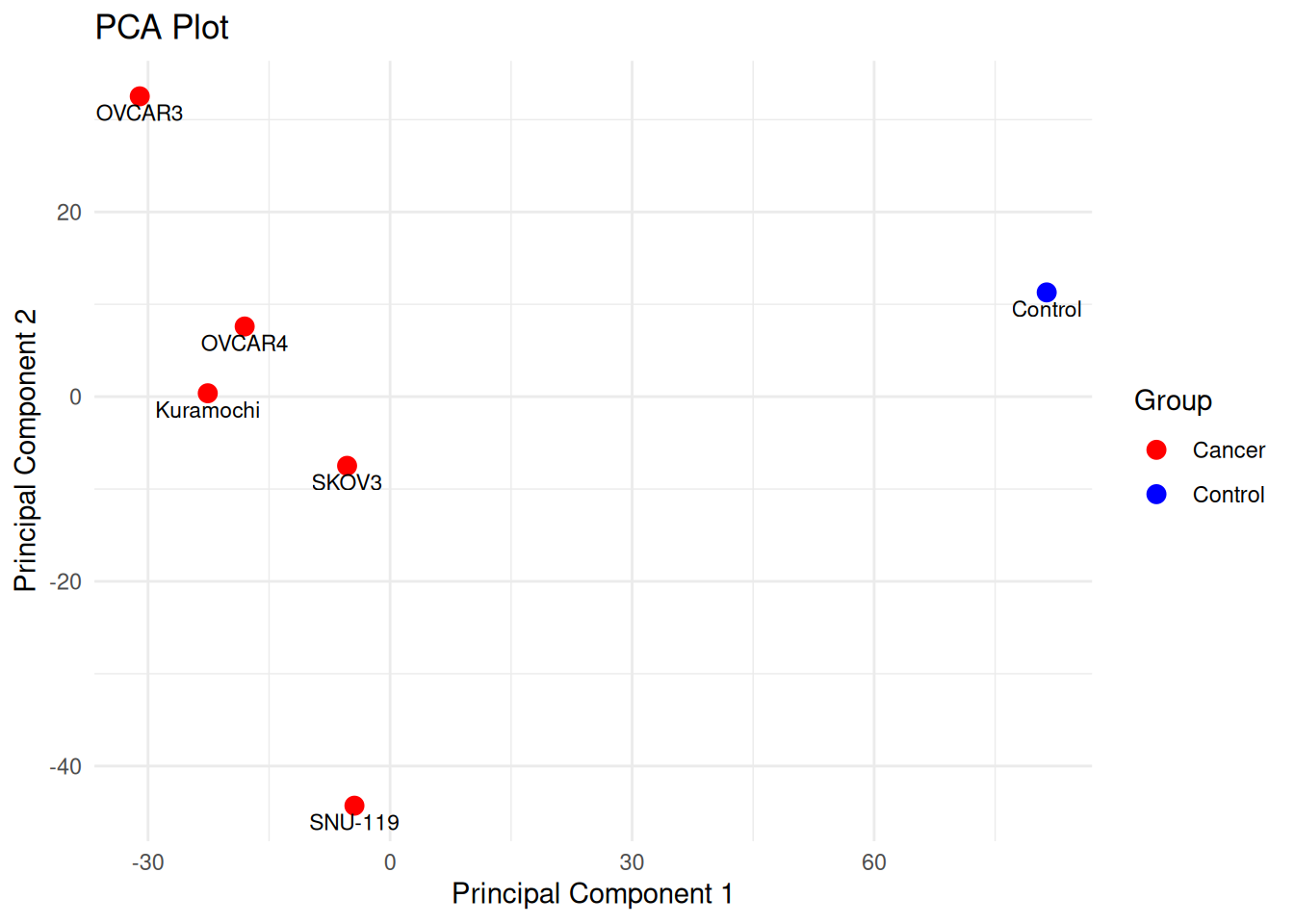
Limitations
Lack of biological replicates for normal samples
Conclusion
By combining volcano plots, bar graphs, and PCA plot, we can dissect the complex transcriptomic landscape of ovarian cancer cells. This structured pipeline not only identifies key regulators but also provides biological insights for downstream validation and hypothesis generation.